Pandas groupby is your your friend, once you get to know it

Categorical variables are the perfect use for Pandas.groupby

Like for my previous post I will be using the arctic penguin dataset as our example dataset.

# Import required packages
import pandas as pd
import numpy as np
import seaborn as sns
from matplotlib import pyplot as plt
df = sns.load_dataset('penguins').dropna()

As we have seen in my previous post, in this dataset we have information for different penguin species, either male or female, living in different islands.

For this example let’s say we are interested in the difference of penguins body mass between the two sexes. Our intuition would tell us that male should be heavier that female but you never know! Maybe in penguins it doesn’t work that way and we could set up a statistical test to check for this hypothesis.

In this post I won’t enter into details in statistical inference so I would simply show some tips and manipulations using Pandas on how you would get around to check for the difference.

The first thing we can do is to use these categorical variables to our advantage. They are a perfect use for Pandas.groupby.

grouped_df = df.groupby(['species', 'sex'])

It is interesting (and a bit counter-intuitive) to notice that the above operation returns a grouped pandas dataframe and it is expecting us to perform some kind of operation onto that object. By itself grouping it like that it’s not so useful, but the grouping is usually then used to calculate grouped statistics (like we will see below).

Interesting use of grouped dataframes

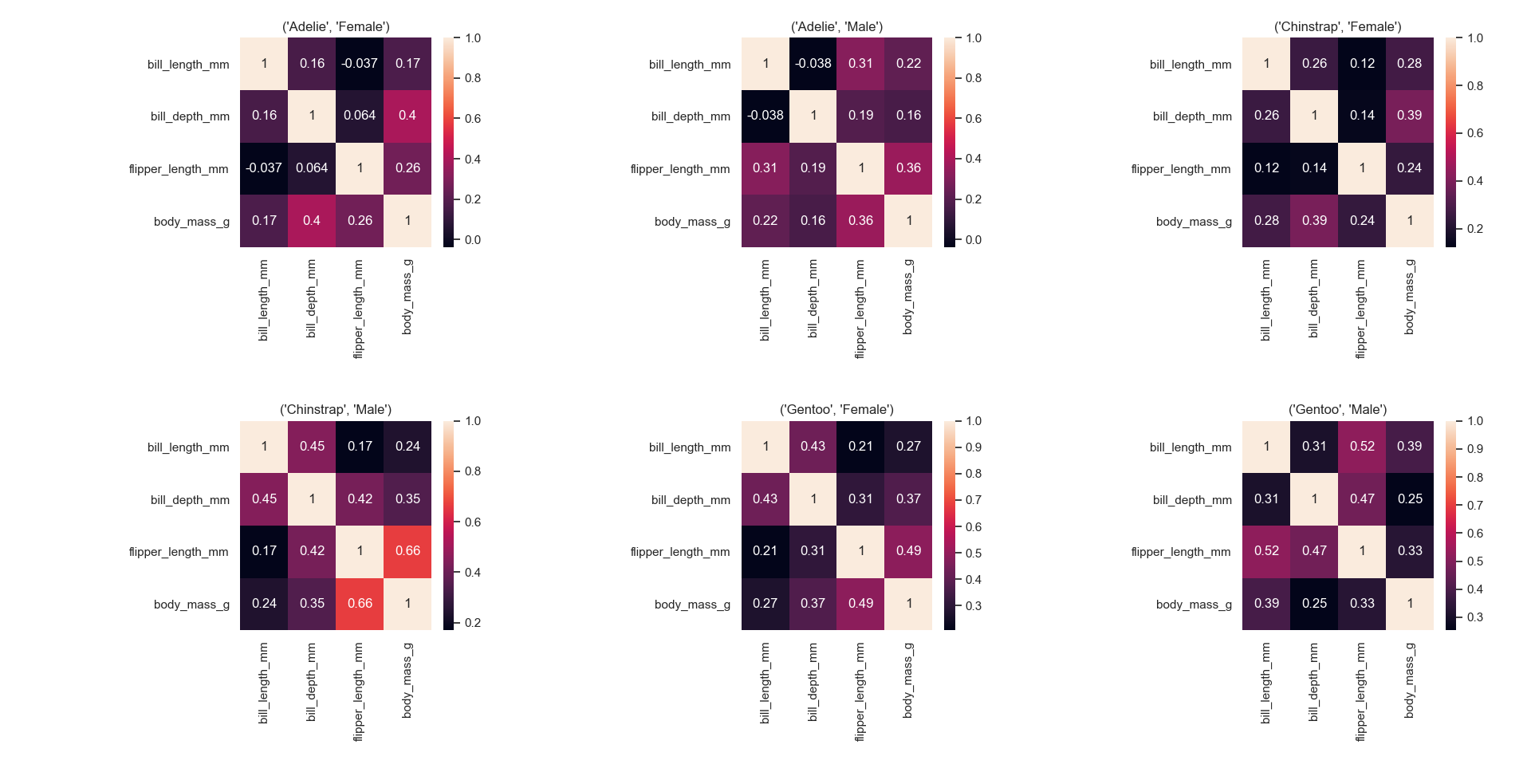
A use for the “simple” grouped pandas dataframe could be to leverage its grouping structure. For example let’s say that we want to perform a certain operation per group that we defined. We don’t really need to calculate grouped statistics but we simply need the groups and the data for each of these groups.

One common application for this could be plotting something per group. Here I unpacked the group and respective filtered dataframe in a loop to create some correlation maps.

number_of_groups = len(grouped_df.groups) # groups is a dictionary so len(dict) will return the number of groups
sns.set(context='notebook') # set style and labels size
f, axes = plt.subplots(2, int(number_of_groups/2), figsize=(10,8)) # create plots grid
for (g, dataframe), ax in zip(grouped_df, axes.ravel()):
    corr_table = dataframe.corr() # calculate correlation table for each group
    sns.heatmap(corr_table, ax=ax, annot=True) # make heatmap of corr table
    ax.set_title(g)
plt.tight_layout()
plt.show()

Calculating grouped statistics

In this case we are interested in checking the difference between male and female penguins body mass in each penguin species. So the first step would be to calculate the mean and standard deviation of the body mass for each of these groups.

A handy function commonly used in pandas is describe.

# calculate stats per group
grouped_df.describe()

But if we know what we want we could ask it specifically instead.

# just returns the mean of any numerical variable
grouped_df.mean()
# get specific stats on specific variable
da = grouped_df.agg({'body_mass_g': [np.mean, np.std]})

Working with MultiIndexed dataframes

What groupby does is use the index of the dataframe to keep track of the groups and the column names to keep track of the calculated statistics. In this case both of these attributes consist of multiple levels: our index will have species and sex and our body_mass_g will have mean and std.

I personally like that it keeps the original labels in the index so we can always refer back to it using strings instead of numbers, using loc:

# access specific values using loc
# while  for single level index/columns you just need on argument
# for multilevel we need to specify each level
da.loc['Adelie', 'Female']['body_mass_g', 'mean']

The above code will return the calculated mean body mass value for female penguins of the Adelie species.

Working with multiple levels for several groups

# since selecting is easier using columns that indeces
# transpose to get categories as variables instead of indeces
daT = da.T
# get high hierarchy categories and loop through them
for species in daT.columns.levels[0]: # get the 3 species in this case
    # Here we calculate the body mass difference between sexes for each species
    daT[species, 'body_mass_diff'] = daT[species, 'Male'] - daT[species, 'Female']

At this stage we could proceed at testing if the per-species-sex-based body mass difference is statistically significant (which we might cover in the future), but for this post I will stop here.

Use pandas dataframe as matrices

Another way to do something similar to what we have done above is to use a functionality of pandas dataframe that I didn’t know until very recently. Pandas dataframe can be treated as matrices if they have the same amount of entries and shape between them. Let’s see an example in which I calculate the sex body mass difference in this way:

# Create a new dataframe for single sex penguins#
df_m = df[df['sex'] == 'Male'].reset_index().drop('index',axis=1).copy() # make a copy of filtered observations
df_f = df[df['sex'] == 'Female'].reset_index().drop('index',axis=1).copy() # drop old index column

# calculate the mean of every numerical variable after grouping our single-sex dataframes by species
df_diff = df_m.groupby('species').mean() - df_f.groupby('species').mean() # calculate the sex difference of every mean
print(df_diff)

A couple of things to notice from the code above:

1. the .copy() method is useful to make sure you create a new dataframe from the old one. If you don’t include it (or something equivalent), the new object you create with the filtered observations, will just be a special way to refer to the original dataframe and not a truly new object!
2. Althought it’s common, it’s usually better to keep the original index column, instead of dropping it (.drop()), to a record of the operation.
3. I don’t recommend to create multiple dataframes from an original dataframe when we are talking about groups or categories. This is what .groupby() is for. Often (me included) because the functionality of .groupby() is not intuitive, it’s easy to fall into the “create a new dataframe for everything” mindset. Avoid it if it can be done otherwise.

SOURCE

You can find the complete python script used for this post here